Modeling disaggregated DHIS2 data in Power BI without losing your mind

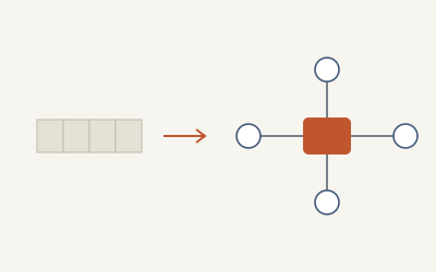
DHIS2 is the reporting backbone for a large share of the world’s public-health programs. It is also, from a modeling point of view, a source that fights you. The data it hands over is already disaggregated — split by age band, sex, facility, site, and period — but it arrives flattened into wide, human-readable exports that were designed to be printed, not queried.

If you point Power BI straight at one of those exports and start writing measures, you will get numbers. They will even look plausible. And a quarter of them will be quietly wrong, because the grain of your table is not what you think it is.

This is the pattern we use to avoid that. Nothing here is exotic — it is disciplined dimensional modeling applied to a source that punishes shortcuts.

The core problem: the export is denormalized, and the disaggregation is trapped in column headers

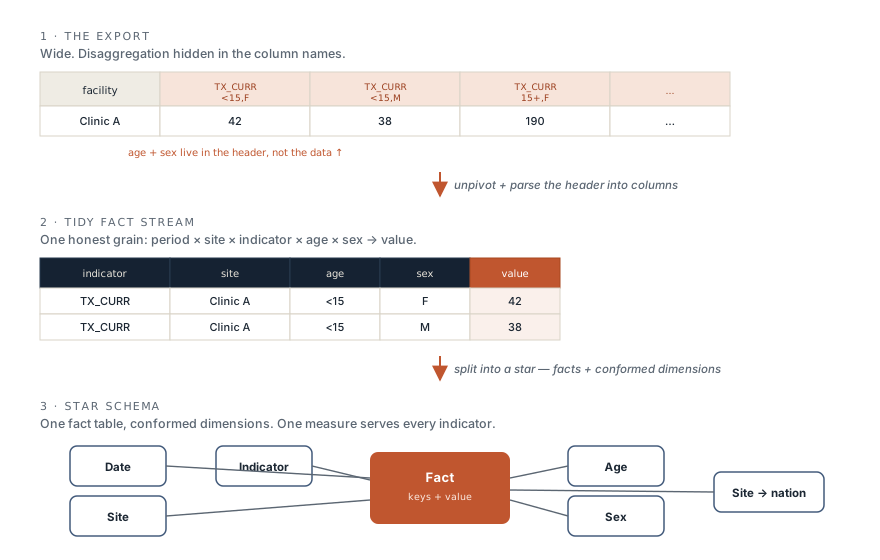
A typical DHIS2 pivot export looks something like this: one row per facility, and a forest of columns like TX_CURR, <15, Female, TX_CURR, <15, Male, TX_CURR, 15+, Female, and so on. The disaggregation you care about — age, sex — is not in the data. It is in the column names.

That means two things are true at once. The table is too wide (dozens of near-identical metric columns), and it is at the wrong grain (one row is a facility-period, but a single fact — one indicator value — is buried inside a cell). Every downstream mistake traces back to this. If you build measures on the wide shape, you end up hard-coding column references, your DAX becomes a wall of SUM('Export'[TX_CURR, <15, Female]), and adding a new age band means rewriting measures instead of loading data.

The fix is to stop treating the disaggregation as structure and start treating it as data.

Step one: unpivot, then parse the disaggregation out of the header

In Power Query, unpivot every metric column so each row becomes a single observation: one indicator, one disaggregation combination, one value. Your forest of columns collapses into two: Attribute (the old header) and Value.

Now the disaggregation is in the Attribute string — TX_CURR, <15, Female — and you parse it into real columns. Split on the delimiter, trim, and you have indicator, age_band, and sex as first-class fields. A few guardrails matter here:

• Parse defensively. DHIS2 header conventions are not perfectly consistent across datasets or program areas. Split on the delimiter, but validate the piece count per row and route anything that does not match an expected shape to an error-inspection query rather than letting it fail silently into a null.
• Normalize category values immediately. <15, < 15, and Under 15 will all show up eventually. Map them to a single canonical set as you parse, so the mess never reaches your model.
• Keep the raw header. Carry the original Attribute string through as a column. When a number looks wrong three weeks later, you want to trace it back to exactly what DHIS2 sent.

After this step you have one long, tidy fact stream at a single, honest grain: period × site × indicator × age × sex → value. Everything good follows from that.

Step two: build the star, not one big table

It is tempting to stop at the tidy flat table and call it done. Don’t. Split it into a star: a central fact table of values, surrounded by conformed dimensions.

• Dimensions: Date (a proper marked date table), Site (with its facility and national rollup as columns, so the hierarchy is real), Indicator, Age, and Sex.
• Fact: one row per observation, carrying only foreign keys and the numeric value.

Two reasons this is worth the extra effort on health data specifically. First, the site hierarchy is the whole game — program teams live in the movement between national totals and a single site’s numbers, and a clean Site dimension with a real national → facility → site hierarchy is what makes that drill-down trustworthy rather than a SUMMARIZE guess. Second, conformed dimensions are what let one measure serve every indicator. Model it once, and the same Date and Site slice TX_CURR, TX_NEW, and viral-load coverage identically. That is the difference between a model that scales as indicators are added and one you rebuild every quarter.

If several DHIS2 datasets feed the same model (a national aggregate and a site-level extract, say), keep them as separate fact tables sharing the same dimensions rather than forcing them into one. A multi-fact star handles different grains cleanly; a single flattened table does not.

Step three: write measures against the grain, once

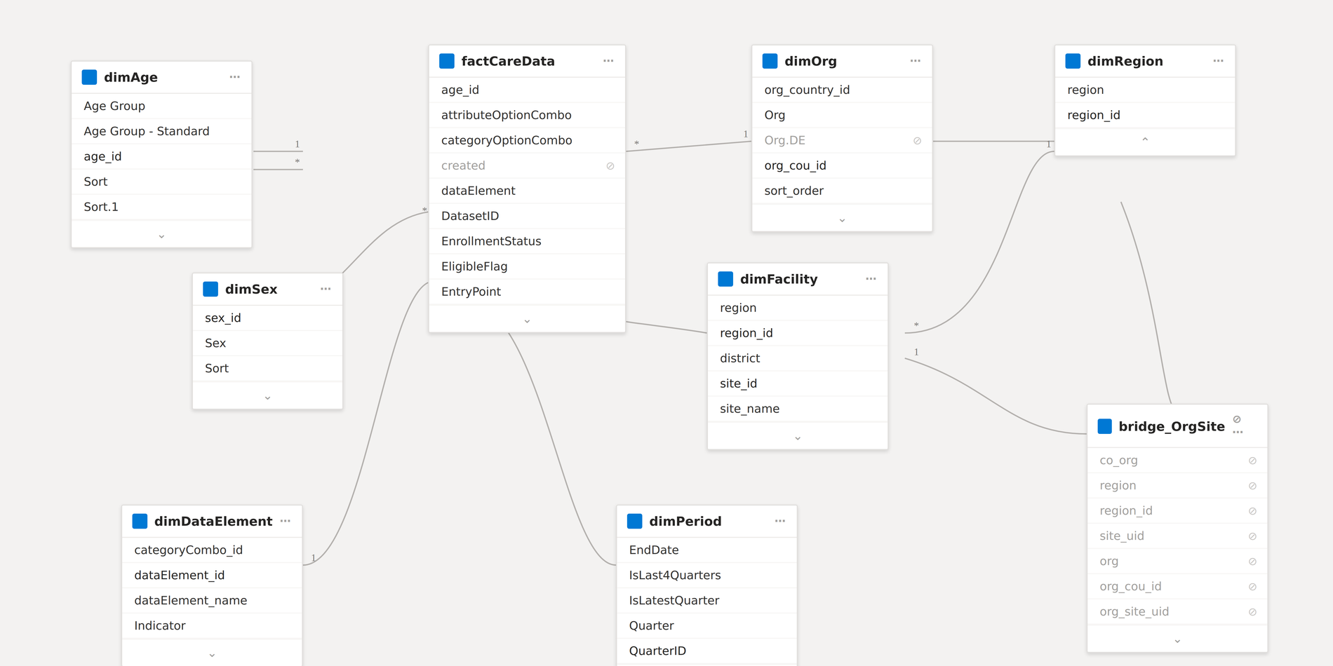
With the star in place, the DAX gets boring — which is the goal. Because the age and sex disaggregations are now dimension columns rather than separate measures, a single base measure plus the filter context does the work:

Total Value = SUM( Fact[value] )

Slice it by Age[age_band], Sex[sex], or Site[level] in the visual, and the number recomposes correctly because the grain is honest. Rates and ratios become one numerator measure over one denominator measure — not a bespoke column per disaggregation. Time intelligence (TOTALYTD, period-over-period) works the first time because you have a real date dimension instead of text periods.

The test of whether you modeled it right: adding a new age band should require loading data, not editing a single measure. If a new disaggregation forces you back into the DAX, the disaggregation is still trapped in structure somewhere upstream. Go find it.

Why this matters beyond the tidiness

It is easy to read all of this as engineering hygiene. It is more than that. On a health program, the model is the argument. When a program lead drills from a national number into one underperforming site and reroutes support there, they are trusting that the drill-down composes correctly — that the site figure and the national figure came from the same honest grain. A model built on a wide export, with disaggregation hard-coded into measures, breaks that trust in ways nobody notices until a decision has already been made on a wrong number.

The star schema is not the interesting part of the work. It is the part that makes the interesting part — the interventions, the reallocations, the questions a team can finally ask of its own data — safe to act on.

This is a field note from our practice. If your team is wrestling a DHIS2 export into something it can actually report on, start a conversation — this is the kind of problem we solve.